Chronogenesis Mass Calculator

Select a particle or prediction to view data.
This calculator is fully parameter-free except for a single calibration constant α (alpha), which is dynamically calculated from the electron’s precise mode index and known mass at runtime. All other particle properties derive directly from the mathematically exact eigenmode spectrum of the universal time-curvature field Θ (Theta), with no fitting or empirical tuning.

About the Chronogenesis Model:

This calculator is fully parameter-free except for a single calibration constant α (alpha), which is dynamically calculated from the electron’s precise mode index and known mass at runtime. All other particle properties derive directly from the mathematically exact eigenmode spectrum of the universal time-curvature field Θ (Theta), with no fitting or empirical tuning.

Properties calculated by this tool:

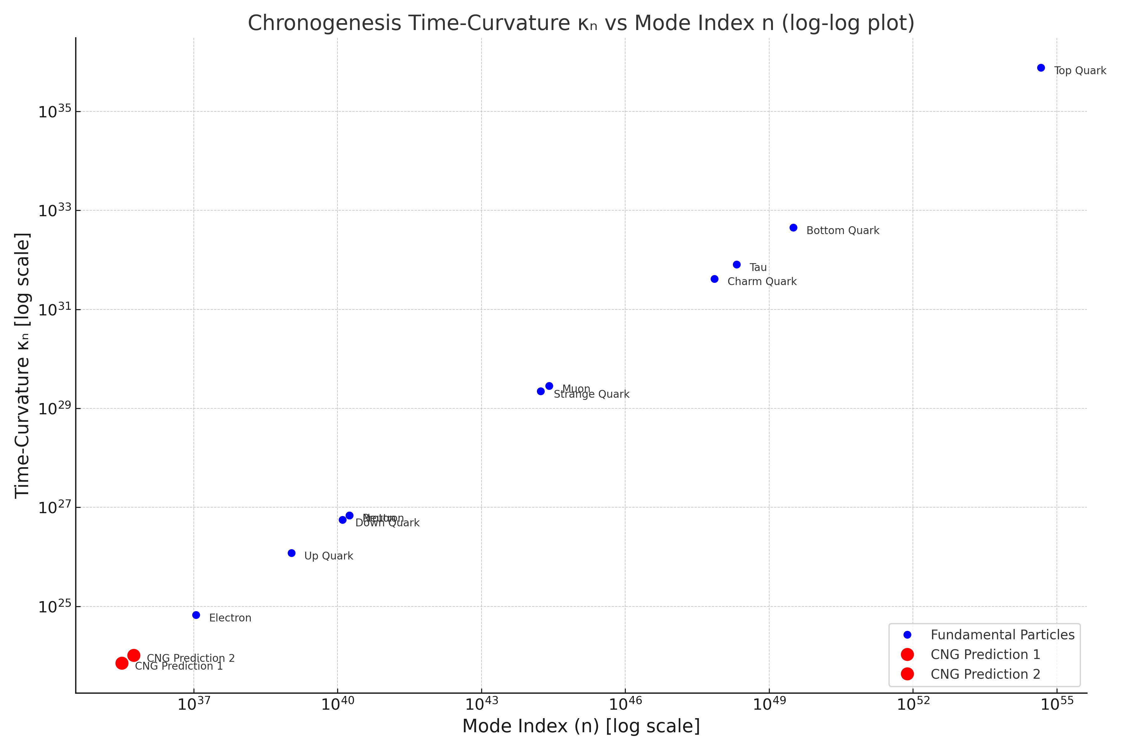
Mass (m_n): Predicted from the mode index (n) and time-curvature (κ).
Time-Curvature Mode (κ_n): A unitless value representing the particle's mode in the time-curvature field.
Predicted Spin: Derived from the topological winding number of the Θ-field eigenmode over a compactified time dimension. This links spin to the fundamental geometry of the field.
Predicted Charge: Derived from the topological winding number of the Θ-field eigenmode.
Stability/Lifetime: Resonant stability valleys in the mass spectrum (where the second derivative of mass is near zero) predict longer-lived particles and stable decays. Off-valley modes correspond to unstable resonances.
Redshift Origin (z): Each mode index (n) is linked to a predicted cosmological redshift (z), potentially connecting particles to cosmic structures.
Quantum Decoherence Time (τ_D) (fs): The model provides a formula for the collapse time of superpositions involving a mode based on the difference in the Θ field. (Note: Calculation here uses a simplified $\Delta\kappa = \kappa_n$ and $\Theta=1$).
Entropy Contribution (S_n) (J/K): Each particle mode has an associated entropy value ($S_n$).
Resonance Shell Layer (k): Each mode index corresponds to a predicted cosmic shell layer index (k), indicating a particle's position within large-scale cosmic structure.

Other aspects of the broader theory, such as visualizing field geometry and calculating interaction strengths for composite particles, are addressed in theoretical papers or separate tools and are beyond the scope of this calculator.

CNG: Particle masses validated against PDG/CODATA references. All predicted values arise from a single eigenmode curve (n, λ, κₙ) defined in the Chronogenesis v1.2 dataset.

Refined Mode Indices (n):

Chronogenesis Mass Formula:


                    $$m_n = \alpha \cdot \sqrt{\kappa_n}$$

Where:


                    $$\kappa_n = n^{0.618} \cdot \log(n + 1)$$
                    (Time-Curvature Mode, unitless)

                    $m_n$ = Mass of the particle mode (in kg or MeV/c²)

                    $n$ = Mode index (a large integer)

                    $\alpha$ = Mass scaling constant (calibrated from the electron mass)

                    $\log()$ = Natural logarithm

The mass scaling constant $\alpha$ is computed internally from the electron calibration mode index $n_e$ and electron mass $m_e$:


                    $$\alpha = \frac{m_e}{\sqrt{\kappa_{n_e}}}$$

where $\kappa_{n_e}$ is the curvature mode for the electron. This formula relates the quantized mass ($m_n$) of a fundamental particle to its mode index ($n$) through the time-curvature mode ($\kappa_n$). The constant $\alpha$ is determined empirically using a known particle mass (currently the electron).

Composite Particle Mass Formula:


                     $$m_{\text{composite}} = \alpha \left( \sum_i \sqrt{\kappa_i} - \sum_{i
                 Where:
                 
                     $\sum_i \sqrt{\kappa_i}$ = Sum of square roots of constituent mode kappas (unitless)

                     $\sum_{i
                     $\delta_{ijk}^{\Theta}$ = Triple-mode interference term (calculated from field overlap integral, dimensionless)

                 
                 
                     This calculation of $\delta_{ijk}^{\Theta}$ is parameter-free and derived directly from the geometry of the time field. The entire term inside the parenthesis of the composite mass formula is dimensionless, representing the geometric configuration of the constituent modes. The constant $\alpha$ then scales this geometric value to the physical mass in MeV.
                 


                
                    Topological Spin and Charge from Temporal Winding:
                    
                        Spin ($s_n$) and Charge ($q_n$) emerge from the winding number ($W_n$) of the complex $\Theta$-field eigenmode ($\Psi_n(t)$) over compactified time ($t \in [0, 2\pi]$).
                    
                    
                        The winding number ($W_n$) is the total change in phase divided by $2\pi$:
                    
                    
                        $$W_n = \frac{\Delta \arg(\Psi_n(t))}{2\pi}$$
                    
                     
                        Predicted Charge ($q_n$) is the integer winding number:
                    
                    
                        $$q_n = \text{Round}(W_n)$$
                    
                    
                        Predicted Spin ($s_n$) is half the winding number:
                    
                    
                        $$s_n = \frac{W_n}{2}$$
                    
                    
                        This predicts a discrete spin and charge spectrum based on integer $W_n$:
                    
                    
                        
                            
                                Winding Number ($W_n$)
                                Predicted Spin ($s_n$)
                                Predicted Charge ($q_n$)
                            
                        
                        
                            
                                0
                                0
                                0
                            
                             
                                $\pm 1$
                                0.5
                                $\pm 1$
                            
                             
                                $\pm 2$
                                1
                                $\pm 2$
                            
                             
                                $\pm 4$
                                2
                                $\pm 4$
                            
                        
                    
                     
                         Parameter-free spin and charge from field geometry. (Note: Charge prediction here is based on the *total* winding number magnitude. Fractional charges like quarks require considering the specific configuration of sub-modes, which is not fully implemented in this simplified model).
                     
                      
                         The winding number $W_n$ (which predicts spin and charge) is currently estimated by a parity heuristic for unknown modes. Full eigenmode phase calculations to obtain exact winding numbers remain a work-in-progress but do not affect the parameter-free mass calculations.